David DeStephano dd2948, Connor Goldman cg3112, Sarah Munro sim2128, RuiJun Chen rc3179 Dec 5, 2019

Motivation

Human health is inextricably linked to the quality of the air we breath we every day. Outdoor air comprises a significant portion of our lifetime air exposure, and the quality of that air has been declining for some time. Air pollution is increasingly recognized as a factor contributing to global morbidity and mortality, particularly with respect to cardiovascular and respiratory health. In 2018, The World Health Organization released a report stating that:

→ 91% of the world population lived in places where WHO air quality guidelines were not met → Air pollution was estimated to cause 4.2 million premature deaths worldwide in 201 → Reduction in pollution would reduce the global burden of disease from heart disease, stroke, lung cancer, and chronic and acute respiratory diseases

**From WHO

Goals

There is a long way to go in improving ambient air quality, but there is a lot to be gained in doing so. Improved monitoring of factors that influence pollution, and increased awareness of associated health risks can advance the road to recovery. Through this project we strive to:

→ Replicate an air quality monitoring system that could be utilized by a government or health entity → Assess meteorological data as a predictor of air quality → Identify temporal trends, if any → Look for associations between air quality and cardiovascular health

Initial Questions

What meteorological factors are associated with increased PM 2.5 in different sites around Beijing. How are these numbers changing over time?

Our Data

Beijing is one of the industrial capitals of the world, and a notorious source of air pollution. For our primary analyses we looked at a dataset describing meteorological and air quality data from 12 sites in Beijing, China over the years 2013 - 2017. This data comes from The UCI Machine Learning Repository. Air quality was measured as a concentration of particulate matter 2.5 (PM2.5) and particulate matter 10 (PM10). PM2.5 is associated with greater health risks, because the smaller size (<2.5um) makes it more efficient at penetrating deeper into the respiratory system. For this reason we chose to analyze PM2.5 as the outcome of interest. (https://www3.epa.gov/ttn/amtic/files/ambient/pm25/spec/drispec.pdf).

Our air pollution dataset included the following variables:

No: row number
year: year of data in this row
month: month of data in this row
day: day of data in this row
hour: hour of data in this row
PM2.5: PM2.5 concentration (ug/m^3)
PM10: PM10 concentration (ug/m^3)
SO2: SO2 concentration (ug/m^3)
NO2: NO2 concentration (ug/m^3)
CO: CO concentration (ug/m^3)
O3: O3 concentration (ug/m^3)
TEMP: temperature (degree Celsius)
PRES: pressure (hPa)
DEWP: dew point temperature (degree Celsius)
RAIN: precipitation (mm)
wd: wind direction
WSPM: wind speed (m/s)
station: name of the air-quality monitoring site

For our secondary analyses, we sought to isolate any associations between air quality and health outcomes in Beijing. We modeled acute myocardial infarction (AMI) as the outcome using the dataset from Liu et al.. The data was collected by the public health information center of Beijing, and includes AMI hospital admissions in Beijing for each month between January 1, 2013 and December 31, 2016.

The following variables were included:

Gender
Admission date(year)
Admission date(month)
Main discharge diagnosis

Exploratory Analysis

Loading and tidying the data

We loaded the data from csv files obtained from the data archive listed above

files = list.files("./PRSA_Data_20130301-20170228", full.names = TRUE)

all_df = map_df(files, read_csv) %>% 
  bind_rows() %>% 
  janitor::clean_names()

We identified a total of 420768 rows/observations, and a total of 18 variables or columns which include the following: no, year, month, day, hour, pm2_5, pm10, so2, no2, co, o3, temp, pres, dewp, rain, wd, wspm, station. We then wanted to characterize the amount of data present and missing for each variable:

Total amount of data:

colSums(!is.na(all_df))

##      no    year   month     day    hour   pm2_5    pm10     so2     no2 
##  420768  420768  420768  420768  420768  412029  414319  411747  408652 
##      co      o3    temp    pres    dewp    rain      wd    wspm station 
##  400067  407491  420370  420375  420365  420378  418946  420450  420768

Amount of missing data for each variable:

colSums(is.na(all_df))

##      no    year   month     day    hour   pm2_5    pm10     so2     no2 
##       0       0       0       0       0    8739    6449    9021   12116 
##      co      o3    temp    pres    dewp    rain      wd    wspm station 
##   20701   13277     398     393     403     390    1822     318       0

From this, it appears that all observations(rows) have date, time, and station information. The number of complete observations with all variables filled in is 382168 which represents the vast majority of the observations.

In tidying the data, we found there is a column/variable ‘no’ which just seems to count rows, which is not needed and removed. We also changed wd and station into factors, added seasons, and created a variable for seasonal years (since winter spans over two years, this variable was created to only be coded as the year in which winter began). Date and datetime variables were also created.

all_df = 
  all_df %>% 
  select(-no) %>% 
  mutate(
    wd = as.factor(wd),
    station = as.factor(station),
    date = as.Date(str_c(year, '-', month, '-', day)),
    datetime = as.POSIXct(str_c(year, '-', month, '-', day, ' ', "00:", hour,":00")),
    season = case_when(
      (month < 3) ~ "winter", #start of Spring is 3/20
      (month == 3 & day < 20) ~ "winter",
      (month < 6) ~ "spring", #start of Summer is 6/21
      (month == 6 & day < 21) ~ "spring",
      (month < 9) ~ "summer", #start of Fall is 9/22
      (month == 9 & day < 22) ~ "summer",
      (month < 12) ~ "fall", #start of Winter is 12/21
      (month == 12 & day < 21) ~ "fall",
      (month == 12 & day >= 21) ~ "winter"
    ),
    seasonal_year=if_else(month<4 & season=="winter" & year ==2014, 2013,
                          if_else(month < 4 & season=="winter" & year ==2015, 2014,
                           if_else(month < 4 & season=="winter" & year ==2016, 2015,
                            if_else(month < 4 & season=="winter" & year ==2017, 2016, year)))),
    season_and= paste(season, " ", seasonal_year)
  )

Visualizing the missing data over time

missing = all_df %>% 
  select(-year, -season, -seasonal_year, -season_and, -datetime, -month, -day, -hour) %>% #the original data except the ones we know are complete
  is.na() %>% 
  as_tibble() %>% 
  mutate(
    date = all_df$date,
    station = all_df$station
  ) %>% 
  pivot_longer(
    cols = pm2_5:wspm
  ) 

missing %>% 
  ggplot(aes(x =date, y = name, fill = value)) + 
  geom_raster(alpha=0.8) + 
  scale_fill_discrete(name = "", labels = c("Present", "Missing")) +
  labs(x = "Variable",y = "Date", title = "Missing values over time") +
  coord_flip()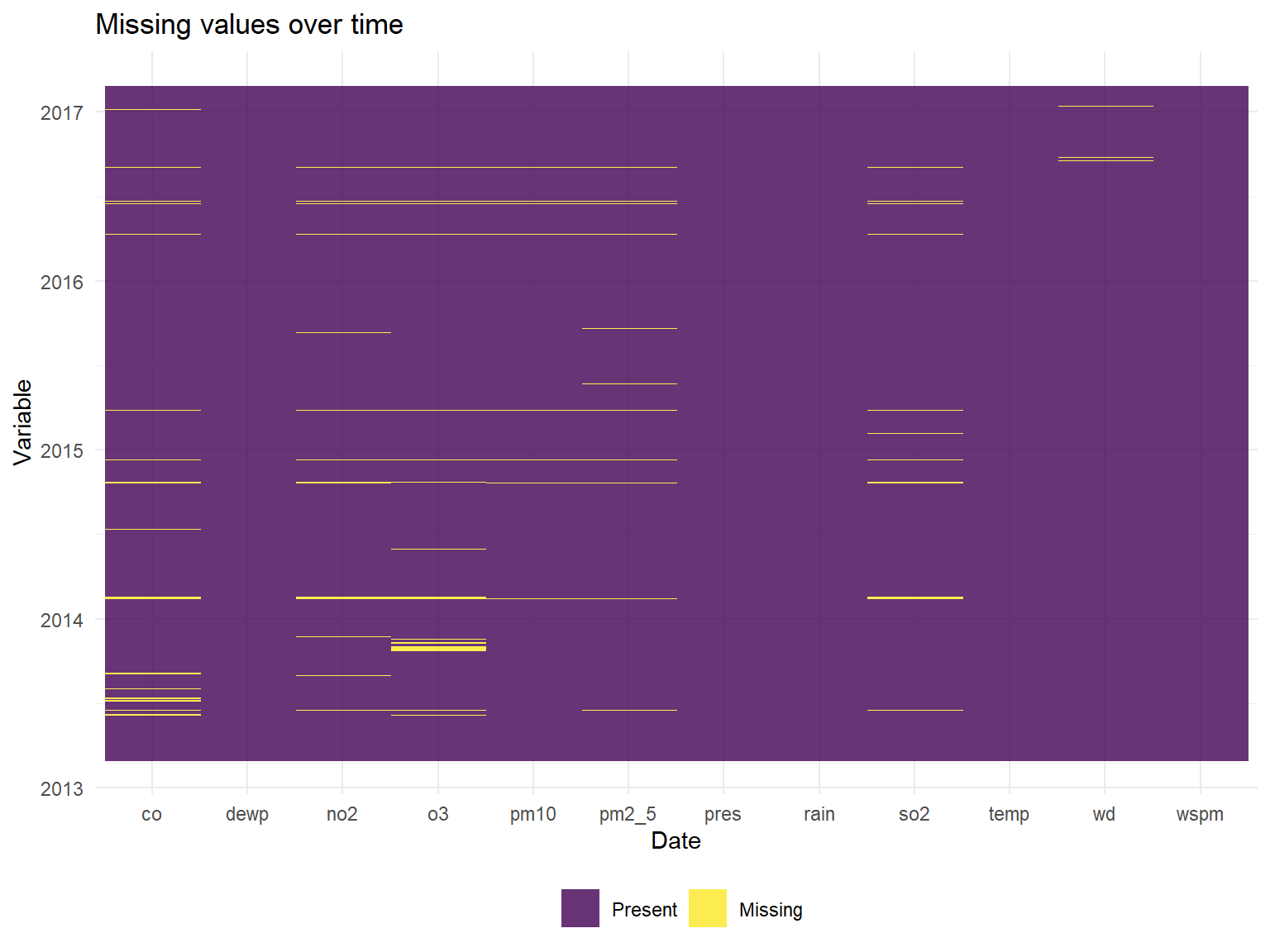

And now visualizing missing data over time across stations:

missing %>% 
  ggplot(aes(x =date, y = name, fill = value)) + 
  geom_raster(alpha=0.8) + 
  scale_fill_discrete(name = "", labels = c("Missing", "Present")) +
  labs(x = "Time",y = "Variable", title = "Missing values over time by station") +
  facet_grid(station~.)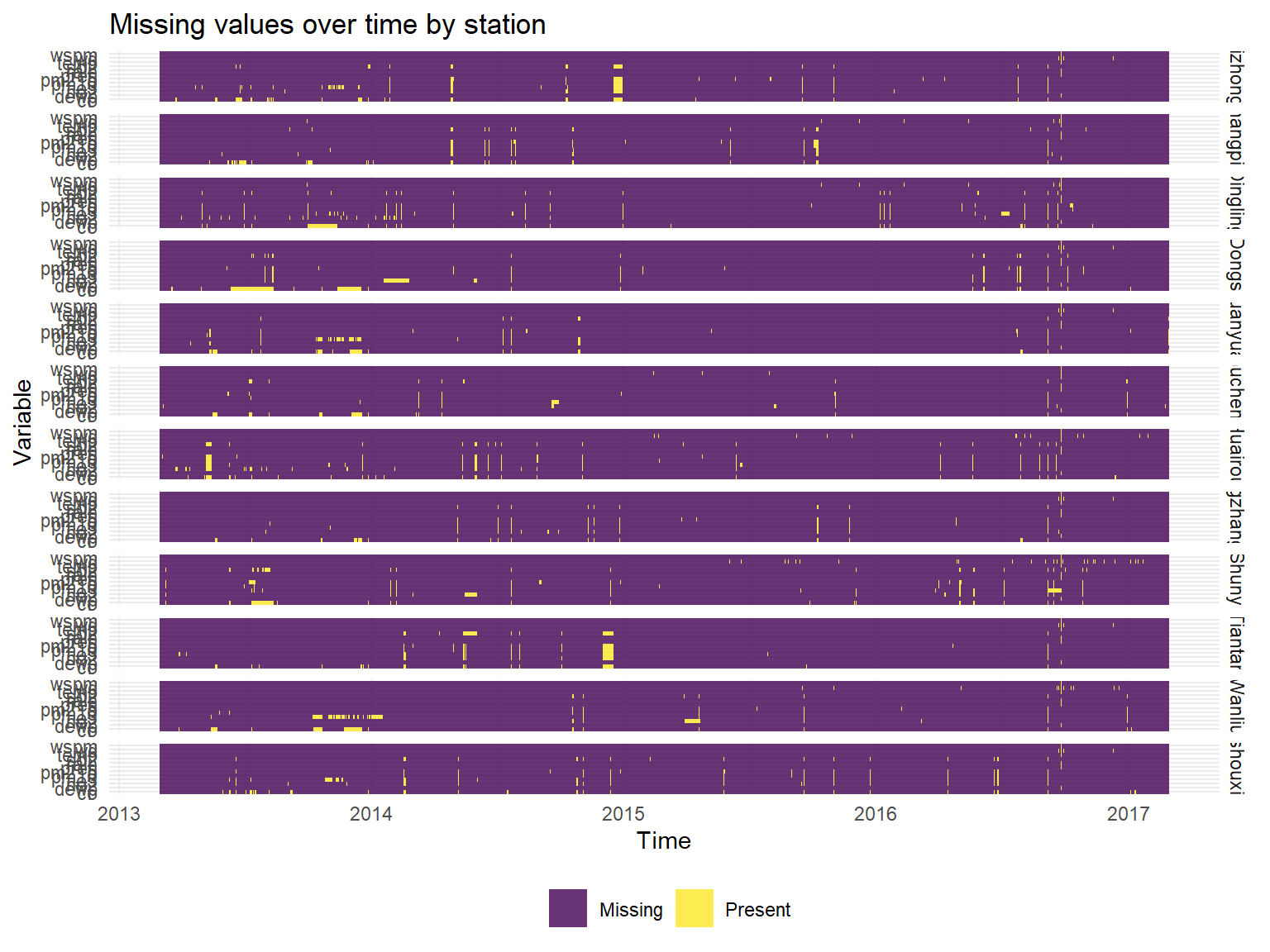

Our primary outcome of interest is PM2.5, and can be summarized as follows:

all_df %>% pull(pm2_5) %>% summary

##    Min. 1st Qu.  Median    Mean 3rd Qu.    Max.    NA's 
##    2.00   20.00   55.00   79.79  111.00  999.00    8739

Looking at PM2.5 over time:

summary

## standardGeneric for "summary" defined from package "base"
## 
## function (object, ...) 
## standardGeneric("summary")
## <environment: 0x000000001ee4f700>
## Methods may be defined for arguments: object
## Use  showMethods("summary")  for currently available ones.

all_df %>% 
  ggplot(aes(x = date, y = pm2_5)) +
  geom_point() +
  geom_smooth()

## `geom_smooth()` using method = 'gam' and formula 'y ~ s(x, bs = "cs")'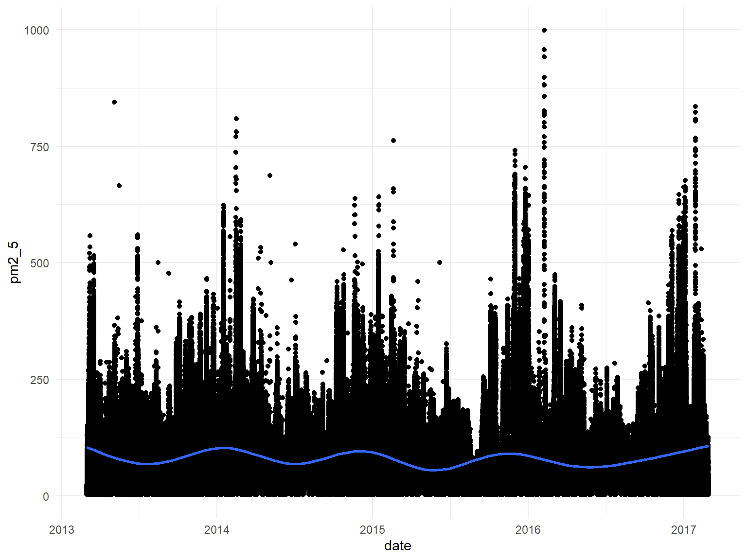

Looking at PM2.5 over time by station:

all_df %>% 
  ggplot(aes(x = date, y = pm2_5)) +
  geom_point() +
  geom_smooth() +
  facet_grid(~station)

## `geom_smooth()` using method = 'gam' and formula 'y ~ s(x, bs = "cs")'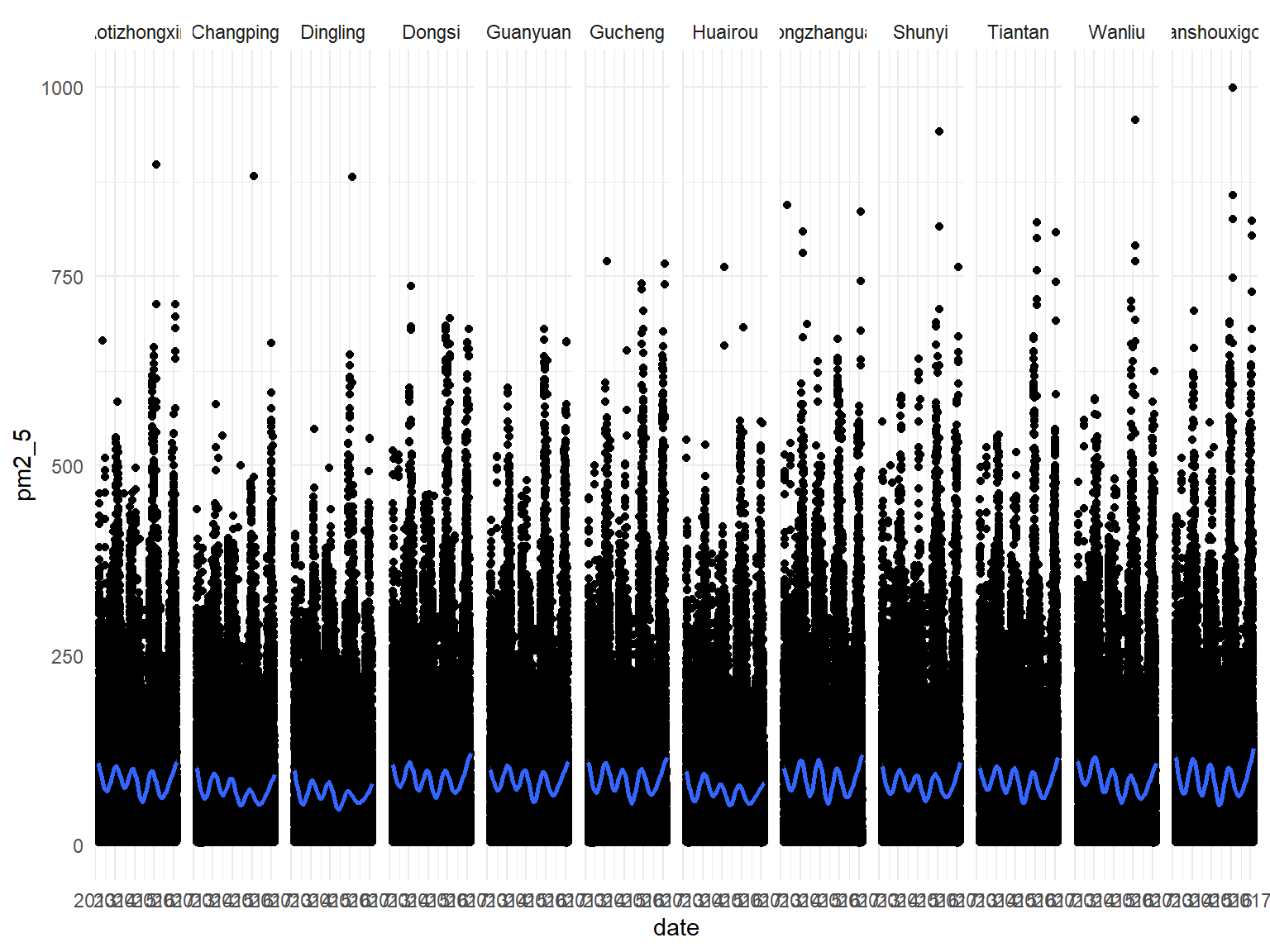

Looking at PM2.5 by seasons:

all_df %>% 
  mutate(
    fct_reorder(season, pm2_5)
  ) %>% 
  ggplot(aes(x = season, y = pm2_5)) + 
  geom_boxplot()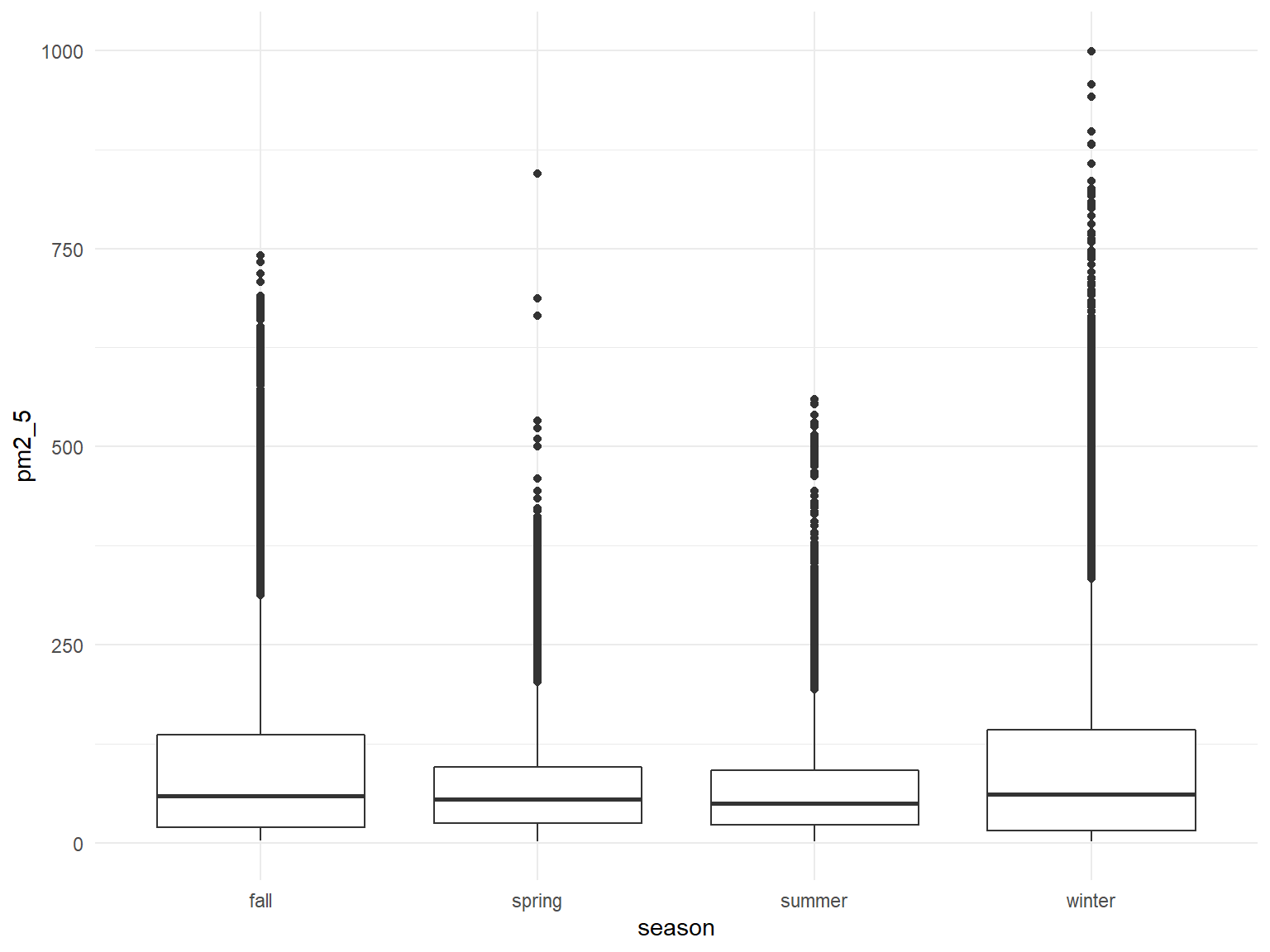

Kind of hard to distinguish, will try limiting scale of y-axis and try a violin plot

all_df %>% 
  mutate(
    fct_reorder(season, pm2_5)
  ) %>% 
  ggplot(aes(x = season, y = pm2_5)) + 
  geom_boxplot() + 
  ylim(0, 250)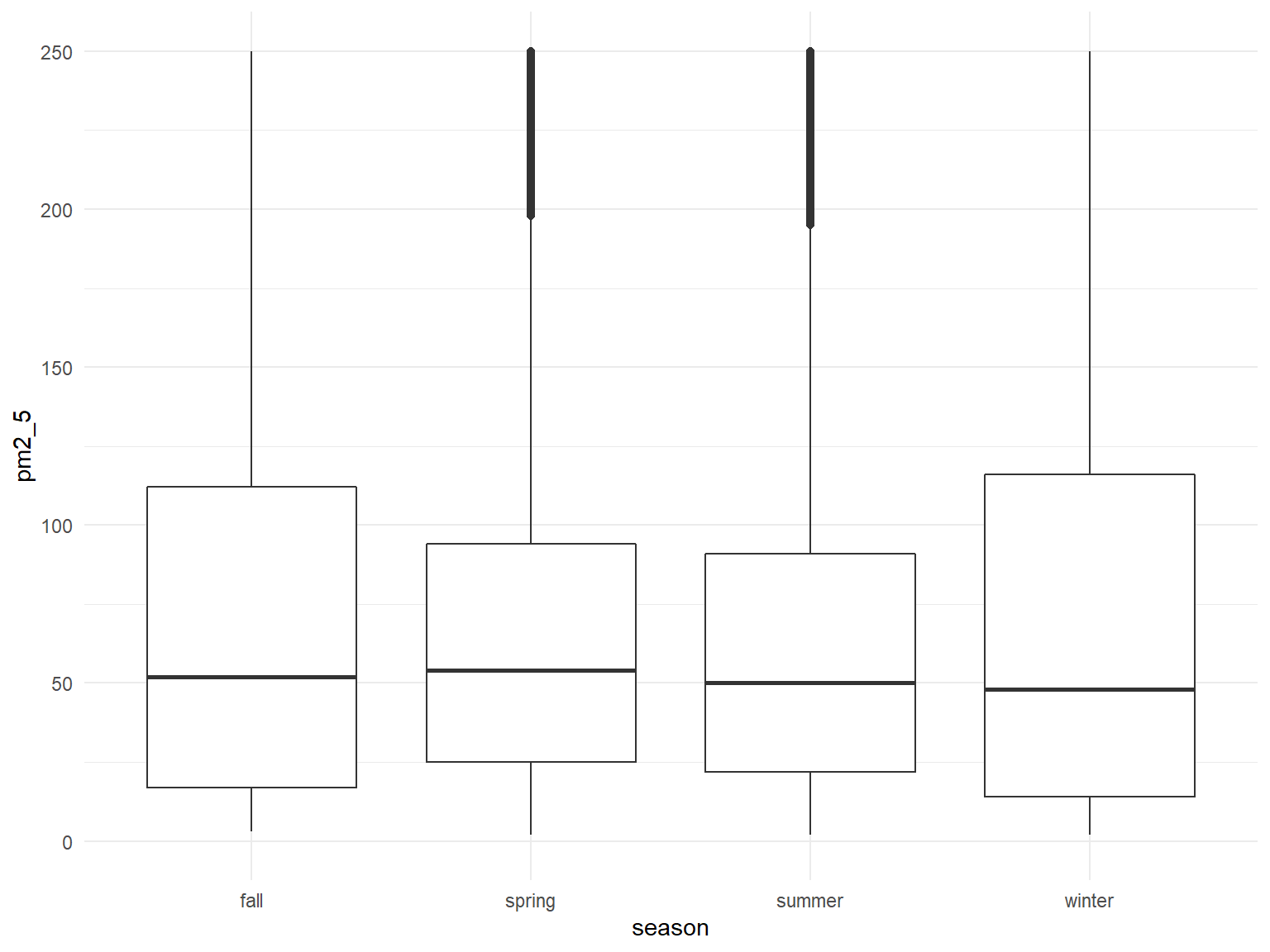

all_df %>% 
  mutate(
    fct_reorder(season, pm2_5)
  ) %>% 
  ggplot(aes(x = season, y = pm2_5)) + 
  geom_violin() + 
  ylim(0, 250)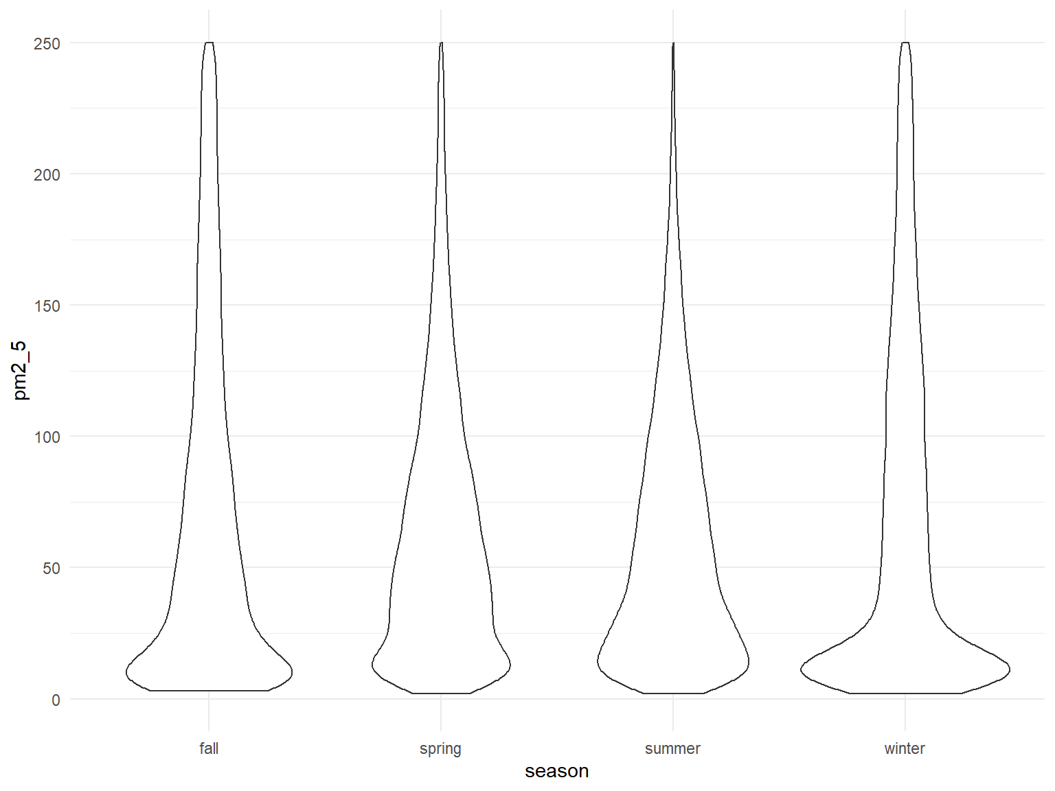

Overall seems fairly similar across seasons, but technically highest in the winter, with a number of very high outlier values as well

Average PM 25 by year for all stations

all_df %>%  
  group_by(year) %>% 
  summarize(avg_pm25=mean(pm2_5, na.rm = TRUE)) %>% 
  ggplot(aes(x=year, y=avg_pm25)) +
  geom_line()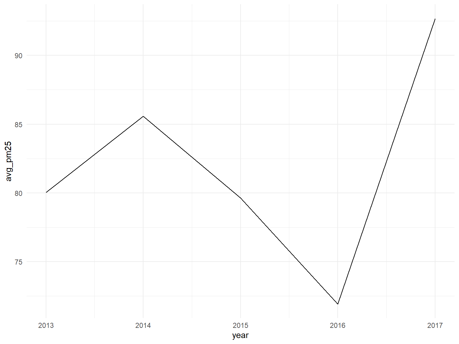

Average PM 25 by year for each station

all_df %>%  
  group_by(year, station) %>% 
  summarize(avg_pm25=mean(pm2_5, na.rm = TRUE)) %>% 
  ggplot(aes(x=year, y=avg_pm25, color=station, group=station)) +
  geom_line()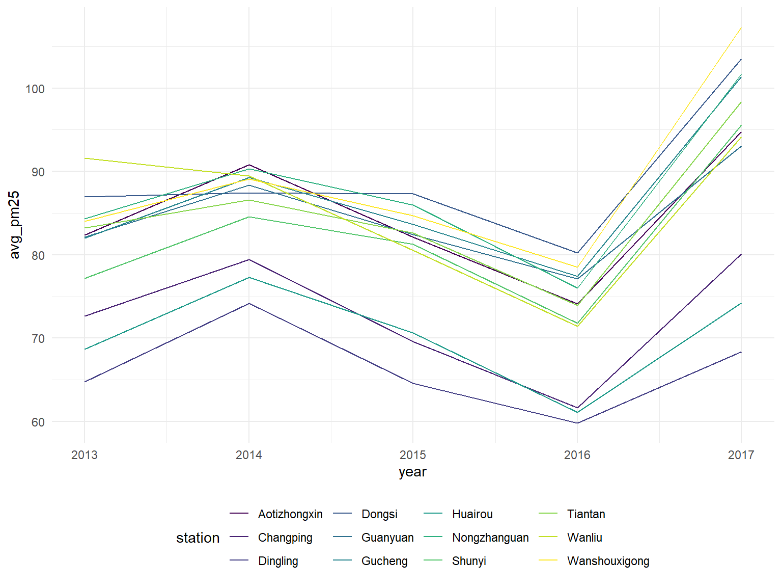

We can see that each individual station seems to follow the same yearly average pm 2.5 trend

Average PM 25 by year and season for each station

all_df %>%  
  group_by(season, seasonal_year, station) %>% 
  summarize(avg_pm25=mean(pm2_5, na.rm = TRUE)) %>% 
  ggplot(aes(x=season, y=avg_pm25, color=station, group=station)) +
  geom_line()+
  facet_wrap(seasonal_year~.) +
  ggtitle("Average PM2.5 by Seasonal Years")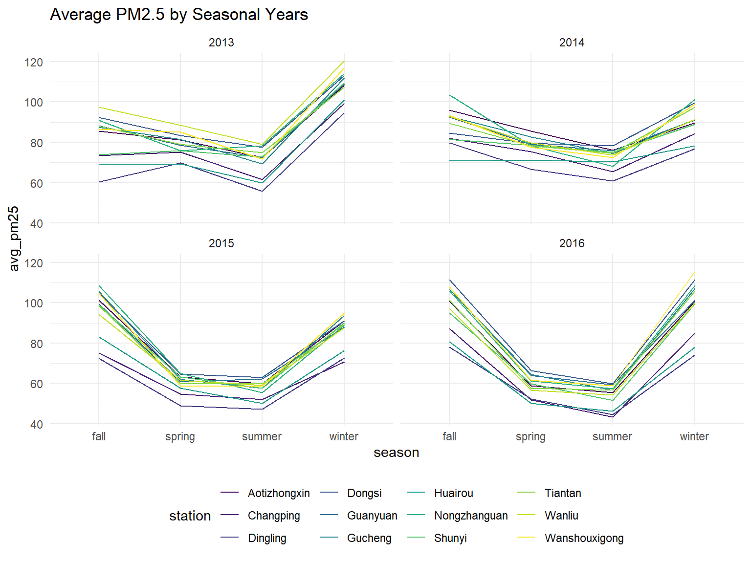

Average PM 25 by year and season for each station

all_df %>%  
  mutate(season_and=factor(season_and, levels = c("spring   2013", "summer   2013", "fall   2013", "winter   2013",
                                                  "spring   2014", "summer   2014", "fall   2014", "winter   2014",
                                                  "spring   2015", "summer   2015", "fall   2015", "winter   2015",
                                                  "spring   2016", "summer   2016", "fall   2016", "winter   2016"))) %>% 
  group_by(season_and, station) %>% 
  summarize(avg_pm25=mean(pm2_5, na.rm = TRUE)) %>% 
  ggplot(aes(x=season_and, y=avg_pm25, color=station, group=station)) +
  geom_line()+
  ggtitle("Average PM2.5 by Seasonal Years") +
  theme(axis.text.x = element_text(angle = 45, hjust = 1))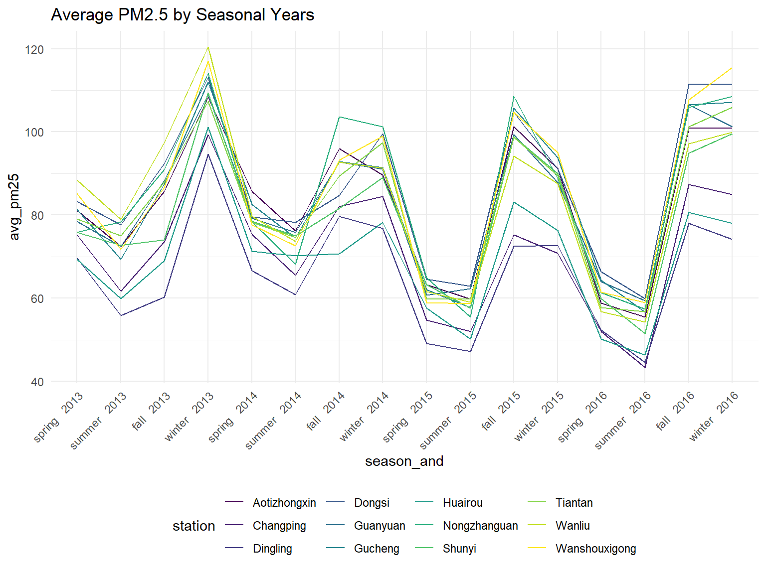

#need to change wspm to CUMULATIVE wind speed for month or direction
all_df %>%  
  filter(station=="Dingling") %>% 
  ggplot(aes(x=dewp, y=wspm, color=pm2_5)) +
  geom_point(alpha=0.10) +
  scale_color_gradient(low="blue", high="red")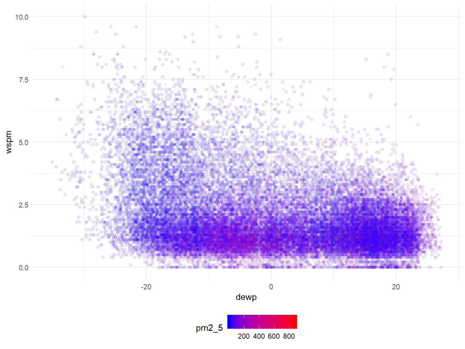

Motherload of all scatterplots (Plotting everything )

Looking at scatter plots of every variable against PM2.5 to look for potential correlation

## Just FYI, this takes a long time to run. And the plots will take up 900MB of memory
#So for now I've set eval=false, but I'm pushing the image it generated, called all_variables_plot.png
par(mfrow = c(4, 5))

vars = all_df %>% select(-pm2_5, -year, -month, -day, -date, -season) %>% colnames()
plots = list()
for (i in 1:length(vars)) {
  plots[[i]] = ggplot(all_df, aes_string(x = vars[i], y = "pm2_5")) + geom_point()
}
do.call(grid.arrange, plots)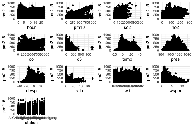

all variables scatterplots

Pearson Correlation Coefficients:

all_df %>% 
  select(-wd, -station, -date, -datetime, -season, -seasonal_year, -season_and, -hour, -year, -month, -day) %>% 
  map(as.numeric) %>% 
  as.data.frame() %>% 
  cor(use = "complete.obs") %>% 
  corrplot(method = "square", addCoef.col = "black", tl.col="black", tl.srt=45, insig = "blank", 
         # hide correlation coefficient on the principal diagonal
         diag=FALSE, number.cex = .7)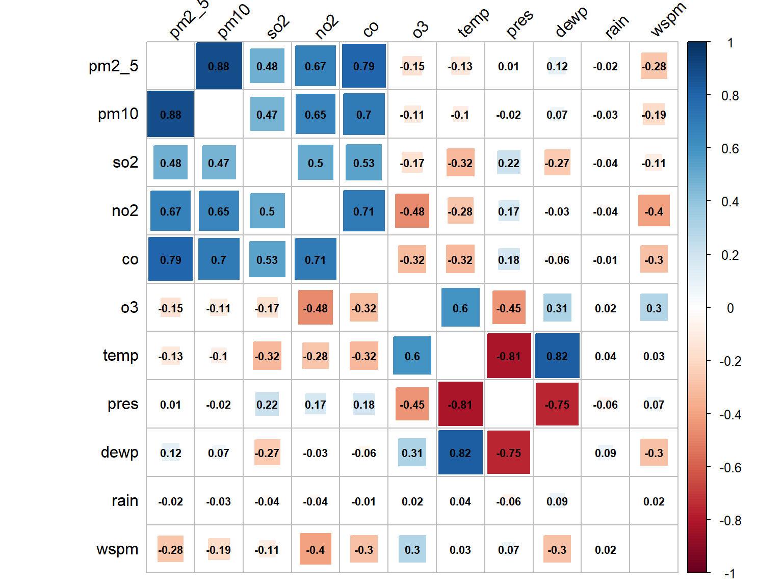

Findings

We looked at correlations between PM 2.5 and the meteorological variables, including dewpoint, windspeed.

We also calulcated spearman’s correlation coefficients to evaluate the inter-relations between air pollutants and weather conditions.

Temperature is correlated with our pollutant concentration, which are all also correlated with eachother, while windspeed has the most effect on decreasing the concentration of these pollutants.

Variables which seem correlated with PM2.5 include (not surprisingly) PM10, but also rain, wind speed, o3 all seem to be strongly correlated. In addition, no2, so2, and possibly temperature, pressure and dew point but in a non-linear fashion

Additional Analysis

Three models were developed for analysis of weather conditions and their association with PM2.5. A multivariable linear regression, a mixed model, and a Mixed Model for Longitudinal Continuous Data were developed to examine the variables of interest.

Almost every variable is significant, however, station, windspeed, season, and windspeed all have high effect sizes. Rain, dewpoint, temp also have moderate effect sizes.

What meteorological variables influence PM 2.5?

Even though predictors are not independent, will model using linear regression before a longitudinal model

###Remove timeseries variables:
reg<-all_df %>% select(-date,-datetime, -month,-day,-hour)

full <- lm(pm2_5 ~ ., data = reg)

tab<-full %>% broom::tidy()
knitr::kable(tab, digits = 3)

term	estimate	std.error	statistic	p.value
(Intercept)	-2976.035	582.399	-5.110	0.000
year	5.810	0.263	22.091	0.000
pm10	0.536	0.001	616.900	0.000
so2	0.110	0.003	32.611	0.000
no2	0.123	0.003	46.056	0.000
co	0.019	0.000	256.446	0.000
o3	0.106	0.001	77.453	0.000
temp	-0.677	0.013	-52.532	0.000
pres	0.299	0.010	30.721	0.000
dewp	1.587	0.009	168.552	0.000
rain	-0.335	0.059	-5.641	0.000
wdENE	-0.385	0.248	-1.550	0.121
wdESE	1.117	0.270	4.136	0.000
wdN	0.547	0.258	2.118	0.034
wdNE	0.125	0.238	0.523	0.601
wdNNE	0.045	0.263	0.172	0.863
wdNNW	0.653	0.274	2.389	0.017
wdNW	-0.278	0.259	-1.076	0.282
wdS	-0.091	0.293	-0.312	0.755
wdSE	-0.696	0.287	-2.425	0.015
wdSSE	-0.276	0.301	-0.916	0.360
wdSSW	-0.147	0.281	-0.523	0.601
wdSW	-1.690	0.264	-6.414	0.000
wdW	-2.462	0.300	-8.199	0.000
wdWNW	-1.394	0.279	-4.993	0.000
wdWSW	-1.639	0.288	-5.687	0.000
wspm	-0.443	0.052	-8.541	0.000
stationChangping	4.431	0.244	18.196	0.000
stationDingling	11.372	0.252	45.135	0.000
stationDongsi	2.663	0.240	11.077	0.000
stationGuanyuan	1.314	0.236	5.576	0.000
stationGucheng	-2.366	0.240	-9.856	0.000
stationHuairou	7.018	0.251	27.939	0.000
stationNongzhanguan	1.994	0.235	8.496	0.000
stationShunyi	6.851	0.244	28.064	0.000
stationTiantan	2.868	0.236	12.169	0.000
stationWanliu	-0.696	0.240	-2.902	0.004
stationWanshouxigong	0.614	0.236	2.604	0.009
seasonspring	-13.535	0.922	-14.687	0.000
seasonsummer	-19.795	0.930	-21.291	0.000
seasonwinter	1.082	0.797	1.358	0.175
seasonal_year	-4.484	0.386	-11.625	0.000
season_andfall 2014	-5.734	0.410	-13.982	0.000
season_andfall 2015	-1.082	0.648	-1.670	0.095
season_andfall 2016	-6.890	0.914	-7.536	0.000
season_andspring 2013	5.622	0.910	6.178	0.000
season_andspring 2014	-1.564	0.639	-2.448	0.014
season_andspring 2015	-6.313	0.394	-16.025	0.000
season_andsummer 2013	4.266	0.911	4.682	0.000
season_andsummer 2014	2.532	0.639	3.962	0.000
season_andsummer 2015	-0.799	0.395	-2.023	0.043
season_andwinter 2013	-0.960	0.747	-1.284	0.199
season_andwinter 2014	-1.359	0.478	-2.843	0.004

Mixed Model

all_df %>% 
  lme4::lmer(pm2_5 ~ year + season + so2 + no2 + co + o3 + temp + dewp + rain + wd + wspm + (1 | station), data = .) %>% 
  broom::tidy() %>% 
  knitr::kable(digits = 3)

term	estimate	std.error	statistic	group
(Intercept)	-1571.860	131.345	-11.967	fixed
year	0.772	0.065	11.843	fixed
seasonspring	-8.107	0.230	-35.256	fixed
seasonsummer	-28.170	0.294	-95.755	fixed
seasonwinter	8.444	0.245	34.490	fixed
so2	0.305	0.005	67.163	fixed
no2	0.728	0.004	207.127	fixed
co	0.038	0.000	390.292	fixed
o3	0.250	0.002	130.725	fixed
temp	-0.866	0.017	-51.273	fixed
dewp	2.241	0.013	175.111	fixed
rain	-1.190	0.085	-14.077	fixed
wdENE	-2.723	0.354	-7.685	fixed
wdESE	2.526	0.386	6.550	fixed
wdN	1.053	0.368	2.858	fixed
wdNE	-1.944	0.339	-5.737	fixed
wdNNE	-2.277	0.375	-6.075	fixed
wdNNW	1.923	0.390	4.933	fixed
wdNW	2.151	0.368	5.839	fixed
wdS	0.739	0.418	1.767	fixed
wdSE	1.815	0.409	4.434	fixed
wdSSE	1.990	0.430	4.631	fixed
wdSSW	1.100	0.400	2.749	fixed
wdSW	-1.142	0.376	-3.038	fixed
wdW	-3.741	0.428	-8.738	fixed
wdWNW	-0.615	0.398	-1.546	fixed
wdWSW	-2.385	0.411	-5.799	fixed
wspm	4.219	0.073	57.781	fixed
sd_(Intercept).station	7.310	NA	NA	station
sd_Observation.Residual	42.580	NA	NA	Residual

Mixed Model for Longitudinal Continuous Data

mixed<-all_df %>% 
  lme4::lmer(pm2_5 ~ year + season + so2 + no2 + co + o3 + temp + dewp + rain + wd + wspm + datetime + (1 | station), data = .) 

mixed %>% broom::tidy() %>% knitr::kable(digits = 3)

term	estimate	std.error	statistic	group
(Intercept)	-50701.822	861.052	-58.884	fixed
year	25.734	0.437	58.854	fixed
seasonspring	-20.355	0.312	-65.209	fixed
seasonsummer	-33.817	0.309	-109.505	fixed
seasonwinter	-7.326	0.366	-20.010	fixed
so2	0.276	0.005	60.756	fixed
no2	0.729	0.004	208.209	fixed
co	0.038	0.000	396.177	fixed
o3	0.252	0.002	132.171	fixed
temp	-0.892	0.017	-52.972	fixed
dewp	2.234	0.013	175.342	fixed
rain	-1.224	0.084	-14.535	fixed
wdENE	-2.557	0.353	-7.248	fixed
wdESE	2.392	0.384	6.229	fixed
wdN	1.125	0.367	3.069	fixed
wdNE	-1.945	0.337	-5.764	fixed
wdNNE	-2.045	0.373	-5.480	fixed
wdNNW	2.130	0.388	5.487	fixed
wdNW	2.283	0.367	6.226	fixed
wdS	0.760	0.416	1.827	fixed
wdSE	1.550	0.408	3.802	fixed
wdSSE	1.945	0.428	4.546	fixed
wdSSW	1.083	0.398	2.719	fixed
wdSW	-1.242	0.374	-3.319	fixed
wdW	-3.541	0.426	-8.305	fixed
wdWNW	-0.271	0.396	-0.684	fixed
wdWSW	-2.137	0.409	-5.220	fixed
wspm	4.256	0.073	58.546	fixed
datetime	0.000	0.000	-57.728	fixed
sd_(Intercept).station	7.346	NA	NA	station
sd_Observation.Residual	42.396	NA	NA	Residual

Linking to health data

Is pm 2.5, season, NO2, or CO associated with CVD?

We used the following articles when preparing to analyze pollutions affect on AMI 1, 2

cvd<-read_csv("./patient_mi_data/patients_mi.csv") %>% janitor::clean_names()

## Parsed with column specification:
## cols(
##   gender = col_character(),
##   `admission date(year)` = col_double(),
##   `admission date(month)` = col_double(),
##   `main discharge diagnosis` = col_character()
## )

cvd2<- cvd %>% 
  group_by(admission_date_year, admission_date_month, gender) %>% 
  summarise(n = n()) %>% 
  rename(year=admission_date_year) %>%
  rename(month=admission_date_month)

pollution<-all_df %>%
  group_by(year, month) %>% 
  summarize(avg_pm2_5=mean(pm2_5, na.rm=TRUE),
            avg_pm10=mean(pm10, na.rm=TRUE),
            avg_co=mean(co, na.rm=TRUE),
            avg_temp=mean(temp, na.rm=TRUE),
            avg_no2=mean(no2, na.rm=TRUE))

model_data <- left_join(pollution, cvd2, by=c("year", "month")) %>% 
  na.omit()

model_data$time <- as.yearmon(paste(model_data$year, model_data$month), "%Y %m")

# Sys.getlocale("LC_TIME")
# 
# model_data<-model_data %>%
#    unite(time, c(month, year), sep = "-", remove = FALSE) %>%
#    mutate(time = parse_date_time(time, "my"), local="English_United States.1252")

Time Series of AMI Hospitalizations Grouping by Gender

model_data %>%  
  ggplot(aes(x=time, y=n, color=avg_pm2_5, group=gender)) +
  geom_line()+
  geom_point(aes(size = avg_co))+
  scale_color_viridis(option = "B")+
  ggtitle("Number of MI's by PM2.5 and Year/Month")

## Don't know how to automatically pick scale for object of type yearmon. Defaulting to continuous.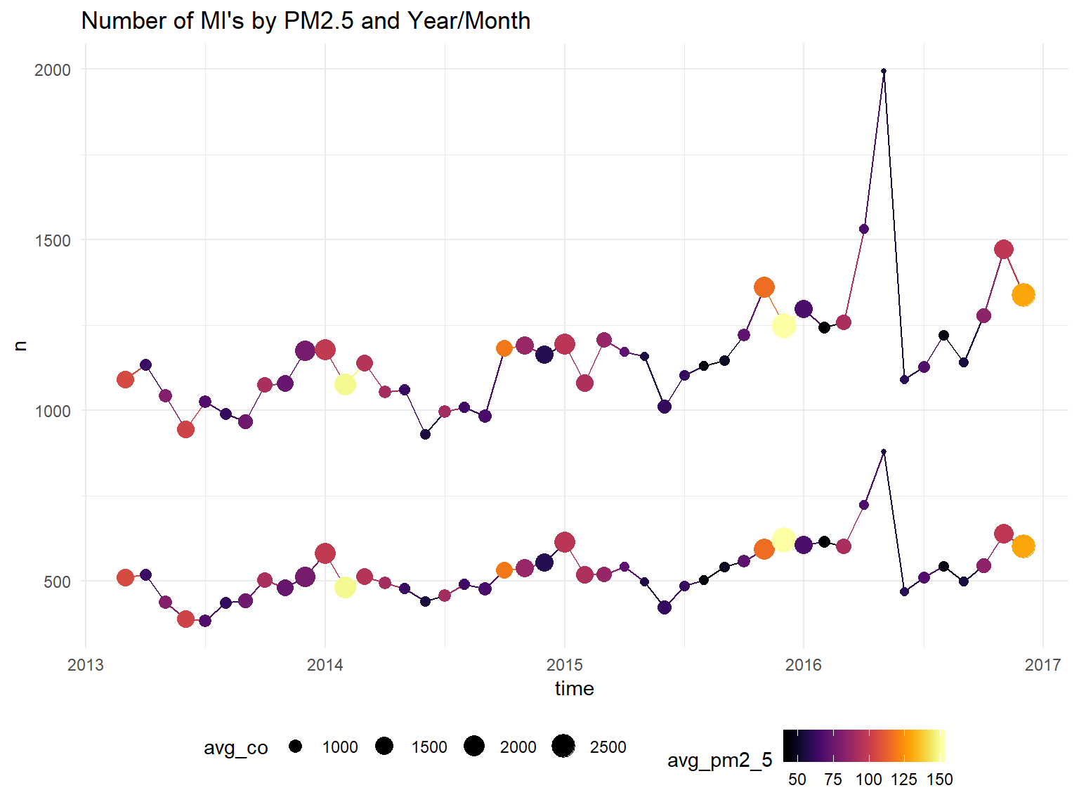

model_data %>%  
  ggplot(aes(x=time, y=n, color=avg_pm2_5, group=gender)) +
  geom_line()+
  geom_point()+
  scale_color_viridis(option = "B")+
  ggtitle("Average PM2.5 by Years")

## Don't know how to automatically pick scale for object of type yearmon. Defaulting to continuous.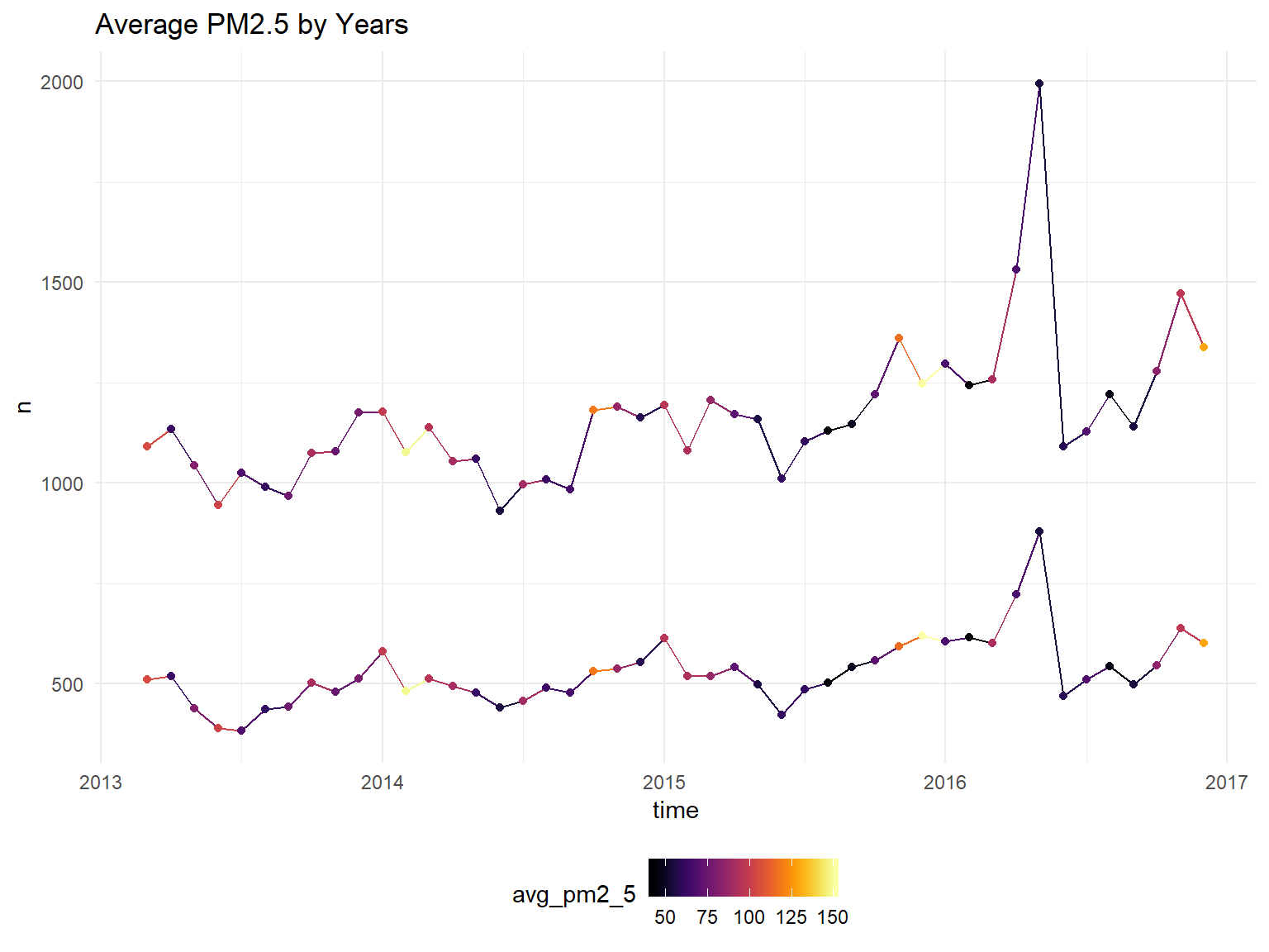

model_data %>%  
  ggplot(aes(x=time, y=n, color=avg_pm10, group=gender)) +
  geom_line()+
  geom_point()+
  scale_color_viridis(option = "B")+
  ggtitle("Number of MI's by PM10 and Year/Month")

## Don't know how to automatically pick scale for object of type yearmon. Defaulting to continuous.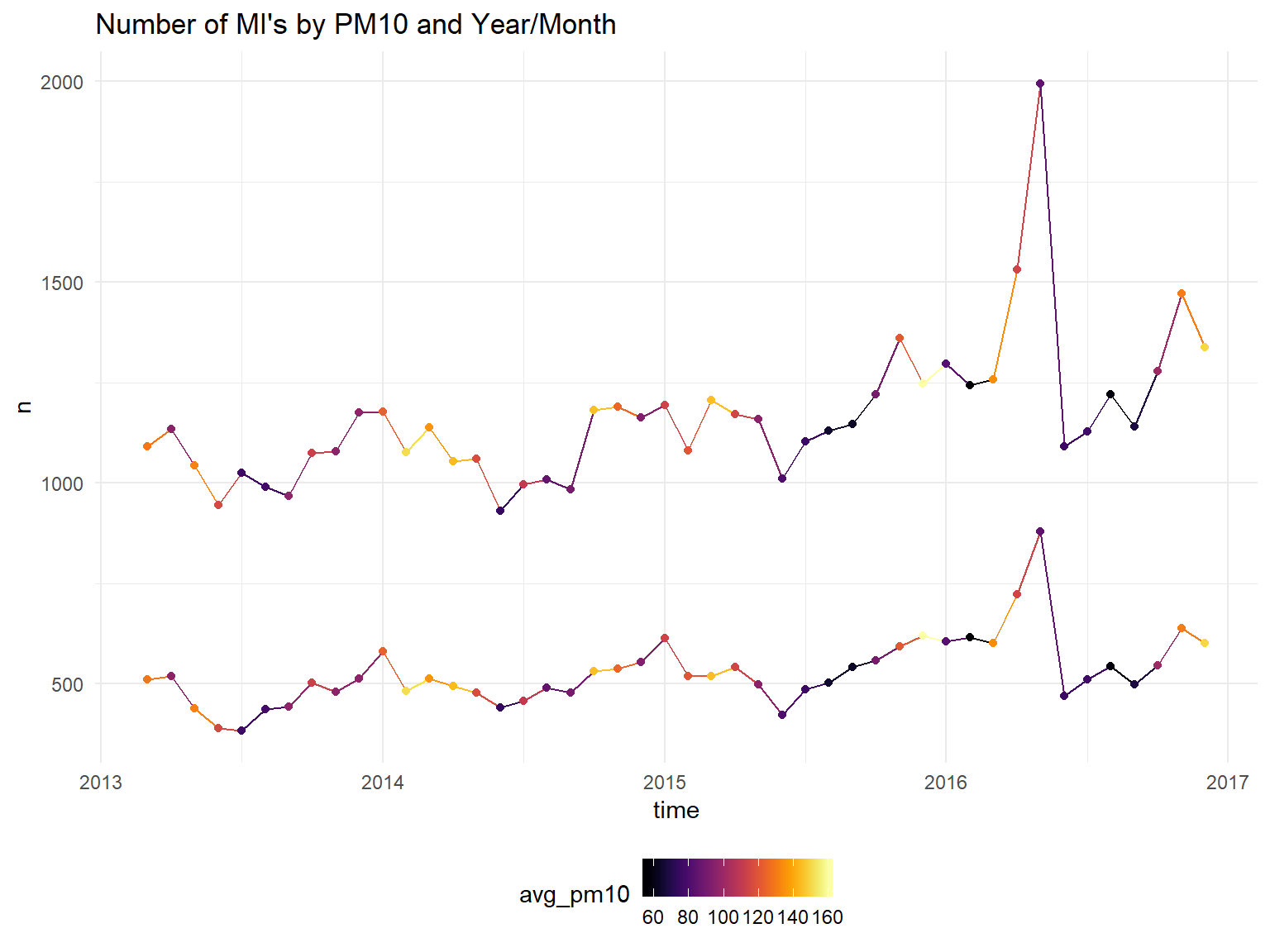

model_data %>%  
  ggplot(aes(x=time, y=n, color=avg_co, group=gender)) +
  geom_line()+
  geom_point()+
  scale_color_viridis(option = "B")+
  ggtitle("Number of MI's by Carbon Monoxide and Year/Month")

## Don't know how to automatically pick scale for object of type yearmon. Defaulting to continuous.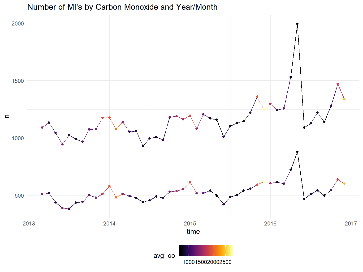

model_data %>%  
  ggplot(aes(x=time, y=n, color=avg_no2, group=gender)) +
  geom_line()+
  geom_point()+
  scale_color_viridis(option = "B")+
  ggtitle("Number of MI's by NO2 and Year/Month")

## Don't know how to automatically pick scale for object of type yearmon. Defaulting to continuous.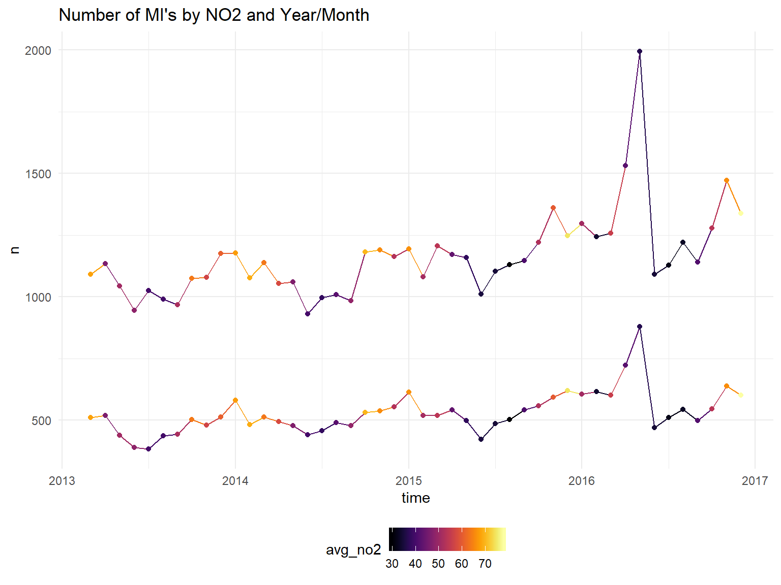

It does appear the hospitalizations are higher in winter months. Unfortunately, we will not be able to draw strong conclusions about the effect pollution on heart attacks since it is so strongly correlated with the month/season. We can try to control for temperature instead of month?

model_data %>%  
  ggplot(aes(x=month, y=n, color=avg_temp, group=gender)) +
  geom_line()+
  geom_point()+
  scale_color_viridis(option = "B")+
  facet_wrap(year~.) +
  ggtitle("Number of MI's by Temperature and Year/Month")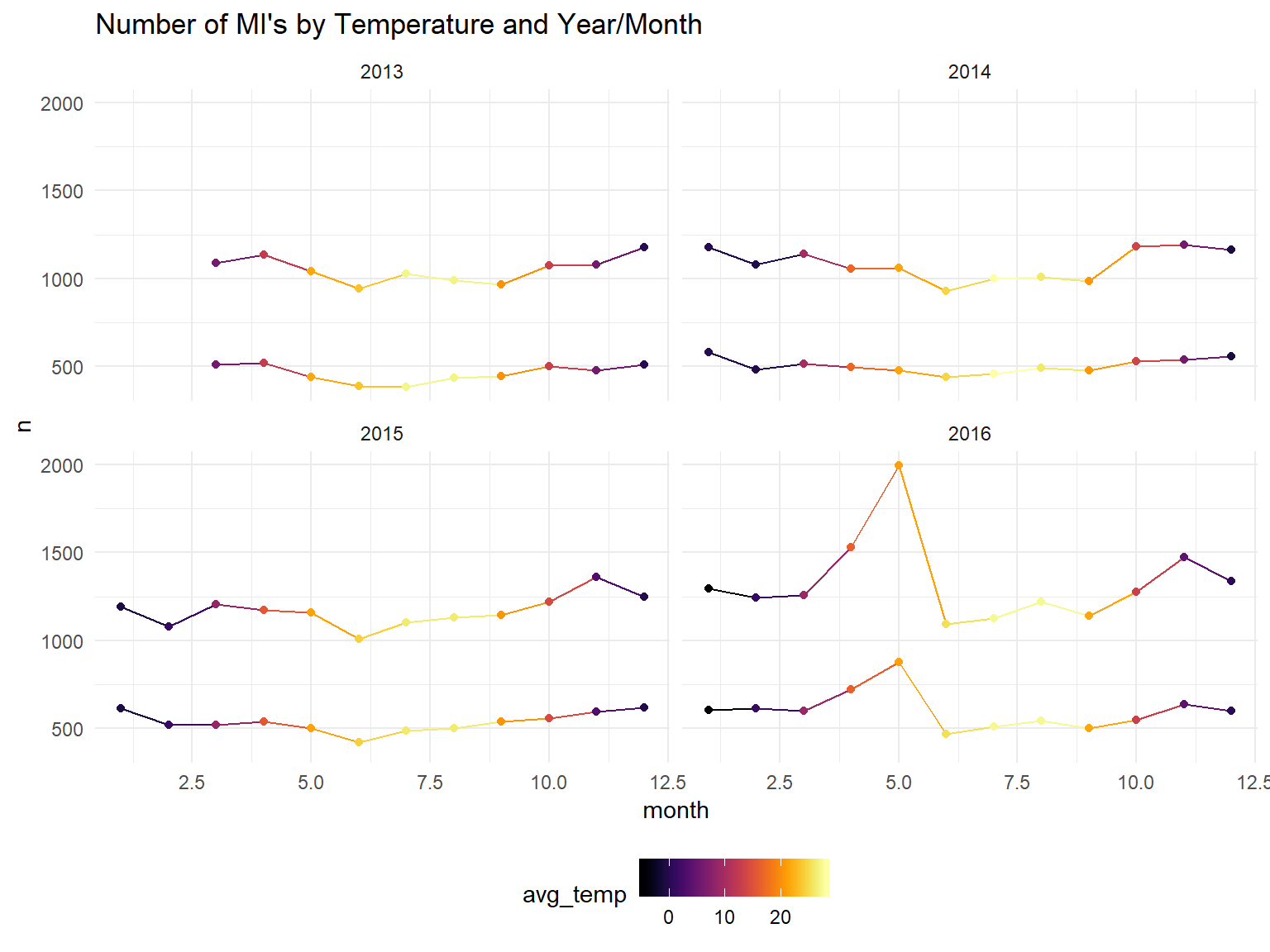

For the analysis we have to use month because we have no data on days of the month to separate analysis into seasons.

The count data we are using is the number of people admitted for MI per month.

Distribution of the counts

count<- cvd %>% 
  group_by(admission_date_year, admission_date_month) %>% 
  summarise(n = n()) %>% 
  rename(year=admission_date_year) %>%
  rename(month=admission_date_month)

count2<-all_df %>%
  group_by(year, month) %>% 
  summarize(avg_pm2_5=mean(pm2_5, na.rm=TRUE),
            avg_pm10=mean(pm10, na.rm=TRUE),
            avg_co=mean(co, na.rm=TRUE),
            avg_temp=mean(temp, na.rm=TRUE),
            avg_no2=mean(no2, na.rm=TRUE))

count3 <- left_join(count, count2, by=c("year", "month")) %>% 
  na.omit() 


count3 %>%
  ggplot(aes(x = n)) + geom_histogram(aes(color = "red")) + labs(title = "Distribution of Counts of MI Data")

## `stat_bin()` using `bins = 30`. Pick better value with `binwidth`.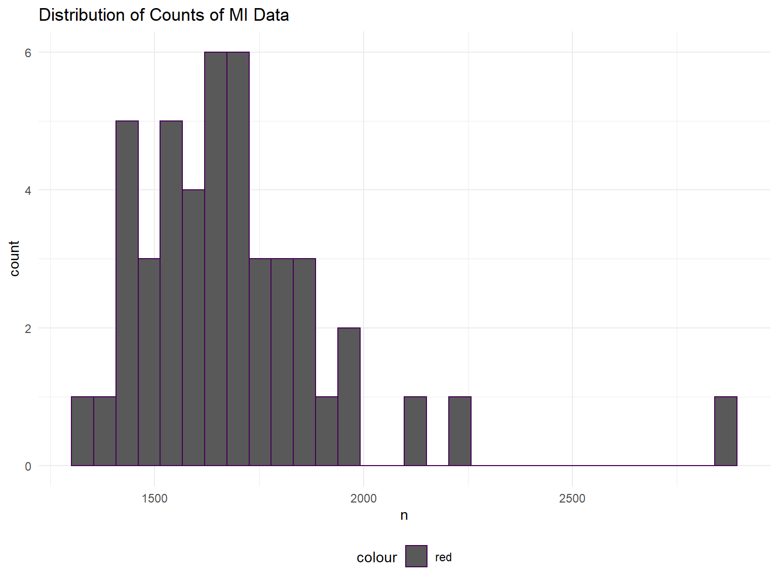

The counts appear to be normally distributed, no overdispersion appears to be present, although we have not formally checked.

We could use a rate for the population of beijing for each year (and month), but from 2014 to 2018, the annual growth rate has been 0.3 percent. Beijing’s population peaked at 21.73 million residents in 2016. Source. For this reason (population numbers have been fairly flat) we decided to just use pure count data.

The count data is in the following format:

head(model_data)

## # A tibble: 6 x 10
## # Groups:   year [1]
##    year month avg_pm2_5 avg_pm10 avg_co avg_temp avg_no2 gender     n time 
##   <dbl> <dbl>     <dbl>    <dbl>  <dbl>    <dbl>   <dbl> <chr>  <int> <yea>
## 1  2013     3     105.     129.   1457.     5.99    67.9 female   511 Mar ~
## 2  2013     3     105.     129.   1457.     5.99    67.9 male    1090 Mar ~
## 3  2013     4      62.1     95.9   903.    12.4     46.3 female   519 Apr ~
## 4  2013     4      62.1     95.9   903.    12.4     46.3 male    1135 Apr ~
## 5  2013     5      81.8    131.    999.    21.7     50.6 female   439 May ~
## 6  2013     5      81.8    131.    999.    21.7     50.6 male    1043 May ~

Should we not include temp? Most is significant when not included.

m1 <- glm(n ~ avg_pm2_5 + avg_pm10 + avg_co + avg_no2  + gender, family="poisson", data=model_data)

tab<-m1 %>% broom::tidy()
knitr::kable(tab, digits = 6)

term	estimate	std.error	statistic	p.value
(Intercept)	6.195519	0.016903	366.540815	0.000000
avg_pm2_5	-0.003976	0.000405	-9.829240	0.000000
avg_pm10	0.002459	0.000321	7.659630	0.000000
avg_co	0.000144	0.000017	8.385587	0.000000
avg_no2	-0.000869	0.000707	-1.229575	0.218856
gendermale	0.789288	0.007736	102.026556	0.000000

Including temp?

m1 <- glm(n ~ avg_pm2_5 + avg_pm10 + avg_co + avg_no2 + avg_temp + gender, family="poisson", data=model_data)

#avg_pm2_5*avg_temp + avg_co*avg_temp

tab<-m1 %>% broom::tidy()
knitr::kable(tab, digits = 3)

term	estimate	std.error	statistic	p.value
(Intercept)	6.558	0.031	210.804	0.000
avg_pm2_5	-0.001	0.000	-1.967	0.049
avg_pm10	0.002	0.000	4.808	0.000
avg_co	0.000	0.000	-1.552	0.121
avg_no2	-0.004	0.001	-5.636	0.000
avg_temp	-0.009	0.001	-13.747	0.000
gendermale	0.789	0.008	102.027	0.000

What about including month and year??

model_data<-model_data%>% 
  mutate(month=factor(month))

m1 <- glm(n ~ avg_pm2_5 + avg_pm10 + avg_co + avg_no2 + month + year + gender, family="poisson", data=model_data)

#avg_pm2_5*avg_temp + avg_co*avg_temp

tab<-m1 %>% broom::tidy()
knitr::kable(tab, digits = 3)

term	estimate	std.error	statistic	p.value
(Intercept)	-159.489	8.401	-18.985	0.000
avg_pm2_5	0.004	0.001	4.550	0.000
avg_pm10	-0.004	0.001	-8.247	0.000
avg_co	0.000	0.000	-1.420	0.156
avg_no2	0.002	0.001	1.588	0.112
month10	-0.056	0.042	-1.328	0.184
month11	0.061	0.022	2.843	0.004
month12	0.058	0.020	2.884	0.004
month2	-0.108	0.033	-3.282	0.001
month3	0.043	0.036	1.209	0.227
month4	0.087	0.047	1.829	0.067
month5	0.135	0.045	3.001	0.003
month6	-0.235	0.043	-5.488	0.000
month7	-0.189	0.051	-3.712	0.000
month8	-0.142	0.042	-3.393	0.001
month9	-0.172	0.039	-4.444	0.000
year	0.082	0.004	19.825	0.000
gendermale	0.789	0.008	102.027	0.000

Including both temp and months/years?

m1 <- glm(n ~ avg_pm2_5 + avg_pm10 + avg_co + avg_no2 + month + year +avg_temp + gender, family="poisson", data=model_data)



tab<-m1 %>% broom::tidy()
knitr::kable(tab, digits = 3)

term	estimate	std.error	statistic	p.value
(Intercept)	-159.650	8.680	-18.393	0.000
avg_pm2_5	0.004	0.001	4.545	0.000
avg_pm10	-0.004	0.001	-7.821	0.000
avg_co	0.000	0.000	-1.371	0.170
avg_no2	0.002	0.001	1.574	0.115
month10	-0.052	0.069	-0.757	0.449
month11	0.063	0.033	1.939	0.053
month12	0.059	0.023	2.604	0.009
month2	-0.107	0.034	-3.161	0.002
month3	0.046	0.047	0.961	0.336
month4	0.091	0.075	1.211	0.226
month5	0.142	0.097	1.456	0.145
month6	-0.228	0.116	-1.963	0.050
month7	-0.180	0.129	-1.400	0.162
month8	-0.133	0.124	-1.077	0.282
month9	-0.166	0.098	-1.699	0.089
year	0.082	0.004	19.206	0.000
avg_temp	0.000	0.004	-0.073	0.941
gendermale	0.789	0.008	102.027	0.000
Interestingly,	all of the	variables a	re significa	nt here.

2016 is an outlier with a large number of MI’s.

2016 may be skewing our result so a seperate set of analyses was completed excluding 2016.

model_data2<-model_data %>% 
  filter(year!=2016)

m1 <- glm(n ~ avg_pm2_5 + avg_pm10 + avg_co + avg_no2 + month + year +avg_temp + gender, family="poisson", data=model_data2)

tab<-m1 %>% broom::tidy()
knitr::kable(tab, digits = 3)

term	estimate	std.error	statistic	p.value
(Intercept)	-112.383	16.142	-6.962	0.000
avg_pm2_5	0.000	0.001	0.205	0.838
avg_pm10	-0.001	0.001	-1.026	0.305
avg_co	0.000	0.000	0.796	0.426
avg_no2	-0.001	0.002	-0.271	0.787
month10	0.203	0.090	2.248	0.025
month11	0.092	0.042	2.186	0.029
month12	0.007	0.027	0.262	0.793
month2	-0.094	0.045	-2.117	0.034
month3	0.119	0.057	2.097	0.036
month4	0.208	0.097	2.156	0.031
month5	0.242	0.128	1.886	0.059
month6	0.119	0.156	0.765	0.445
month7	0.238	0.175	1.358	0.175
month8	0.250	0.167	1.500	0.134
month9	0.173	0.129	1.336	0.181
year	0.059	0.008	7.375	0.000
avg_temp	-0.013	0.006	-2.231	0.026
gendermale	0.788	0.009	85.298	0.000

Now it appears that neither of the two pollution measures are significantly associated with MI.

What if we do not include month and year?

m1 <- glm(n ~ avg_pm2_5 + avg_pm10 + avg_co + avg_no2  + gender, family="poisson", data=model_data2)

tab<-m1 %>% broom::tidy()
knitr::kable(tab, digits = 6)

term	estimate	std.error	statistic	p.value
(Intercept)	6.027276	0.022318	270.067311	0.000000
avg_pm2_5	-0.002491	0.000447	-5.572765	0.000000
avg_pm10	0.001153	0.000374	3.083456	0.002046
avg_co	0.000121	0.000019	6.307927	0.000000
avg_no2	0.002295	0.000778	2.950562	0.003172
gendermale	0.787605	0.009234	85.298203	0.000000

Now all of the variables are significantly associated with MI. This may be the most parsimonious model, but we can not make any causal asumptions.

What if we add interaction of temperature with relevant variables?

m2 <- glm(n ~  avg_pm2_5 + avg_pm10 + avg_co + avg_no2 + gender + avg_temp*avg_pm2_5 + avg_temp*avg_pm10 + avg_temp*avg_co + avg_temp*avg_no2, family="poisson", data=model_data2)

tab<-m2 %>% broom::tidy()
knitr::kable(tab, digits = 6)

term	estimate	std.error	statistic	p.value
(Intercept)	6.255528	0.074958	83.453634	0.000000
avg_pm2_5	-0.000339	0.000779	-0.434447	0.663964
avg_pm10	0.000679	0.000861	0.788775	0.430243
avg_co	-0.000016	0.000037	-0.417864	0.676047
avg_no2	0.000594	0.001743	0.340874	0.733198
gendermale	0.787605	0.009234	85.298203	0.000000
avg_temp	0.002728	0.003612	0.755368	0.450028
avg_pm2_5:avg_temp	0.000021	0.000053	0.384101	0.700903
avg_pm10:avg_temp	-0.000027	0.000052	-0.528269	0.597312
avg_co:avg_temp	-0.000009	0.000003	-3.020829	0.002521
avg_no2:avg_temp	0.000010	0.000104	0.095229	0.924133

We can see that all of the variables, apart from the interaction of temperature and CO are no longer significant. It is possible that this study does not have enough power to assess interactions, since we only have month wide data. This is especially true when we filter out 2016.

We will assess model fit by comparing our two most probably models in ANOVA

The full model formally has a better fit, but is also more difficult to intepret.

anova(m1,m2, test = "Chisq")

## Analysis of Deviance Table
## 
## Model 1: n ~ avg_pm2_5 + avg_pm10 + avg_co + avg_no2 + gender
## Model 2: n ~ avg_pm2_5 + avg_pm10 + avg_co + avg_no2 + gender + avg_temp * 
##     avg_pm2_5 + avg_temp * avg_pm10 + avg_temp * avg_co + avg_temp * 
##     avg_no2
##   Resid. Df Resid. Dev Df Deviance  Pr(>Chi)    
## 1        62     328.33                          
## 2        57     241.77  5   86.562 < 2.2e-16 ***
## ---
## Signif. codes:  0 '***' 0.001 '**' 0.01 '*' 0.05 '.' 0.1 ' ' 1

Discussion

After extensive visualization and modeling of variables in our data we have gained a number of valuable insights regarding Beijing air quality from 2013-2017. Of the meteorological predictors we examined, rain, wind, and temperature were found to be negatively associated with PM2.5. This is consistent with previous findings. There were also strong seasonal variations in air quality, likely attributable to changes in the aforementioned weather variables. PM2.5 was highest across winter and fall seasons, and lowest across spring and summer seasons, for all stations. In concert with the natural decrease of temperature and wind during the winter, we suspect that an upsurge in coal heating also explains the seasonal PM2.5 increase. Visualization of temporal trends demonstrates that pollution was highest in 2014 and 2017, and drastically lower in 2016. The lower average in 2013 may be partially attributable to the absence of data from two winter months. The stations with average PM2.5 concentrations greater than or equal to 100 ug/m3- Nongzhanguan, Dongsi, Wanshouxigong, Gucheng- were all located near the city center. Peripheral stations had relatively lower concentrations.

Further integration of health data into our analysis produced results that were somewhat less anticipated. Visual examination of plots gives the impression that there are slightly more MIs with increasing pollutants, including PM2.5, PM10, CO, and NO2. However, when modeling the data with Poisson regression it appears that there are no significant associations between PM2.5, PM10 when using the full dataset. We considered the year 2016 as an outlier and removed it from the model, when only including pollutants and gender, the pollutants were significant and positive (except PM 2.5), but we can not draw strong conclusions.

This could be due to our model specifications. When examining the count distribution, the data appeared to be more Gaussian than poisson, and we may not have include the correct combination of covariates and interaction terms. A further problem was that we did not have acces to days of the month, so seasonal variables could not be used for the analysis, only months.

In the medical literature, clinicians have noted an increase in cardiovascular disease, and MIs in particular, during the winter months dating back to the 1930s. This finding has been validated across multiple databases and sites worldwide. However, the pathophysiologic mechanism driving this association remains somewhat unclear. Recent evidence has hypothesized that winter weather conditions and cold temperatures may induce physiologic stress including sympathetic activation (thereby increasing blood pressure and heart rate), hypercoagulability, inflammatory markers, and infection which mediate this increase in cardiovascular disease. Age and gender interactions with season and weather have been described. Although we do not find a clear association between air quality, temperature and incident MIs, there may be a number of possible explanations. We used air quality and cardiovascular outcome data from a single city, Beijing, which collected data from multiple sites across the city. Given that the cardiovascular data was collected from a subset of hospitals in Beijing, as not all hospitals were equipped with electronic health records during that time, and we do not have information on the data validation process or quality metrics (including the notable spike in MIs in 2016), the MI data may not be representative of either the general population in Beijing or the population around the air quality reporting sites specifically. In addition, atherosclerosis and coronary artery disease is generally a chronic, multi-factorial process where both risk and mitigating factors such as medications accumulate over time, so there may be unmeasured cardiovascular risk factors or other residual confounding to better explain the MI patterns in Beijing.

Project Report

Motivation

Goals

Related Work

Initial Questions

Our Data

Exploratory Analysis

Loading and tidying the data

Total amount of data:

Amount of missing data for each variable:

Visualizing the missing data over time

And now visualizing missing data over time across stations:

Looking at PM2.5 over time:

Looking at PM2.5 over time by station:

Looking at PM2.5 by seasons:

Kind of hard to distinguish, will try limiting scale of y-axis and try a violin plot

Average PM 25 by year for all stations

Average PM 25 by year for each station

Average PM 25 by year and season for each station

Average PM 25 by year and season for each station

Motherload of all scatterplots (Plotting everything )

Pearson Correlation Coefficients:

Findings

Additional Analysis

What meteorological variables influence PM 2.5?

Even though predictors are not independent, will model using linear regression before a longitudinal model

Mixed Model

Mixed Model for Longitudinal Continuous Data

Linking to health data

Is pm 2.5, season, NO2, or CO associated with CVD?

Time Series of AMI Hospitalizations Grouping by Gender

Distribution of the counts

Should we not include temp? Most is significant when not included.

Including temp?

What about including month and year??

Including both temp and months/years?

2016 is an outlier with a large number of MI’s.

What if we do not include month and year?

What if we add interaction of temperature with relevant variables?

We will assess model fit by comparing our two most probably models in ANOVA

Discussion